EP 1130-2-500
27 Dec 96
units out simultaneously since all units are typically not in operation simultaneously even when all
are available. Values assumed for this example are shown in Table F-2.
f. Since the repair costs and opportunity costs can occur in future years, the analysis
requires discounting the costs in each year to the base year. A discount rate of 8.5% is used in
this example. The current year Federal discount rate should be used in an actual evaluation,
(8.00% in FY94).
g. The evaluation problem is modeling the possible pathways or sequences of
performance that each component for each unit can take, including resetting of the risk after
failure of a component. In addition, the
model must be flexible to deal with
situations with multiple power units and
multiple components. The model must
account for:
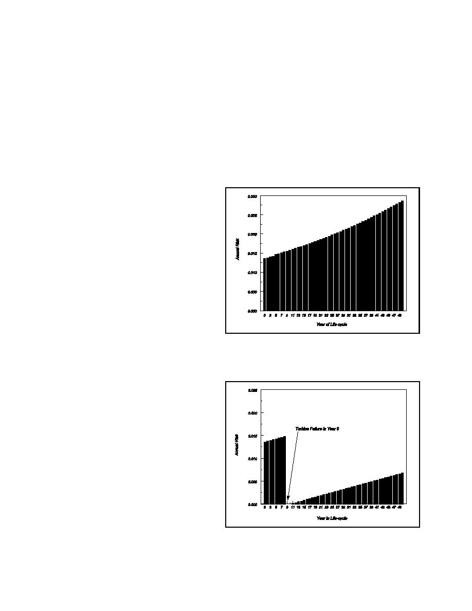
(1) the change in reliability of a
component (increases in risk) over
time from the start of the analysis,
(2) the changed reliability of a
repaired component, (see Figure F-
3),
(3) the possible change in
degradation rate of the repaired
component,
Figure F-2: Non-linear Risk Function
(4) the present value of component
repair costs when a component
fails,
(5) the present value of foregone
project outputs (energy and
capacity) when some units are out
of service due to component
unsatisfactory performance,
(6) the time necessary to repair
components,
(7) the present value of regular
O&M costs while repairs are
undertaken, and
(8) the present value of regular
O&M costs after repairs are made.
h. Once these values are
determined, they can be used in a risk-
Figure F-3: Life-cycle Risk with One Repair
F-3


 Previous Page
